KOI-134: A giant planet with extreme TTVs
-
 by
Shellface
by
Shellface
Well, time to put all this to paper. I've been working on this for most of this week, so this'd better get somewhere!
I noticed KOI-134 because it is marked as a false positive in the KOI catalogue for no obvious reasons, as the transits seem fine and there are no obvious eclipses. Though the parameters listed in the catalogue match the transits to the eye (the period given is 67.5952229 days, and the transit depth is 5276 ppm; this gives a companion radius of ~1.1 Rjup, for the KIC radius), the data validation reports model several periods that appear to attempt to model some, but not all, of the transits independently. The TCERT report is similar, but it is important to note that the periodicities fitted seem to misrepresent some of the transit times (see in particular page 4). If the transits were perfectly periodic, this would not happen - the best-fit period would be an integer multiple of the real period, and all of the transits would fall perfectly in line with that model. These oddities suggested to me that this KOI has large TTVs, which would explain the poor modelling because the Kepler pipeline has no real treatment for TTVs, so it diverges onto whatever models provide a more satisfactory fit, regardless of their likelihood. This behaviour can be seen for KOI-142 (Kepler-88), which is a system where large TTVs on the transiting planet were used to unambiguously solve the system parameters (see Nesvorny et al. (2013)). As KOI-142 is the only other case I know of where the Kepler pipeline fails so badly, this loosely suggests that KOI-134.01 may have TTVs of similar magnitude. Surprisingly, this does not seem to have been recognised in literature at all; I expect this is due to this KOI being marked as a false positive.
Though, obviously, not much can be learned from such incorrect models, it at least appears that the centroids are well-behaved and do not shift during transits, indicative of the transits are on-target.
What really tipped me off on the system, though, was this thread by troyw on the old talk, which I happened across by coincidence. TTVs can clearly be seen, and it can be readily identified that they are substantially larger than the transit length (which is almost 12 hours!), and that they are obviously sinusoidal. I will throw caution to the wind here and say that this can't not be a planetary system - for such a long orbital period, TTVs of such a (relatively) short period and enormous amplitude can only be produced by resonant planetary system; a stellar mass for the KOI would require a stellar mass for the peturber, which is not conceivably stable due to the long period of the transiter (and the RVs do not agree with such a high mass; see below). Any more exotic solutions are incompatible with the excellent transit morphology.
(I did ask troy a few questions about those plots a bit ago, but it looks like he's not around)
So, why is this KOI listed as a false positive? I must say, I still cannot give a definitive answer - nothing in the catalogue shows indication of a false positive scenario over poor modelling, and nothing of the sort appears at CFOP, either. I must assume that the false positive status of the KOI is simply down to poor interpretation of the lightcurve, in a model without TTVs. Though false positive interpretation in the KOI catalogue is often very good, it seems to be incorrect here.
Speaking of CFOP - discussion there involves several spectroscopic observations. Though I am obligated to respect their limits on the redistribution of information as much as possible, I will say that the RVs discussed indicate little RV variation over a few hundred m/s, which suggests a companion mass below, say, 10 Mjup. The observation of v sin i = 12 ± 2 km/s is also valuable. There is also some recognition of the TTVs, though this could only be based on a few quarters as it was several years ago, now. As Geoff Marcy said:
This system remains a mystery, in need of both radial velocity measurements over time and of modeling.
Though this was said over 3 years ago, I believe it still stands today.
Let us turn to the lightcurve. Overall, the transits provide the largest variations present. That said, there is some degree of short-period variability. These variations are complex, and though not satisfactorily modelled by simple sinusoids, they generally follow a quasi-periodicity of ~7.3 days. As the star is reasonably late-type, this is best interpreted as a rotational period. The exceptionally small amplitude of the variability (<1000 ppm) suggests very little spot presence, which is consistent with the star having a post-main-sequence surface gravity determined spectroscopically and via the KIC (though the KIC is generally not very reliable for surface gravities), and a noted lack of chromospheric emission its spectra. As we have knowledge of the star's rotational period and v sin i, we can give an inequality for the stellar radius following
sin i = 0.01977(...) * Prot *(v sin i /R)
where sin i is the star's rotational inclination with respect to the line of sight. sin i = 1 gives a lower limit to the stellar radius, which thus gives R > ~1.73 Rsol. This supports the idea that the star is fairly evolved; given the KIC effective temperature of 6038 ± 105 K, it is perhaps not yet a subgiant, but certainly can no longer be considered an F-dwarf. Additionally, a star of such an evolutionary state cannot be much larger than 1.73 Rsol, which indicates sin i ~ 1, so that the stellar rotational axis is close to alignment with the planetary orbital axis, which is called spin-orbit alignment. As the long period of the planet precludes tidal interaction (and the star probably lay above the Kroft break, so that it would be unable to strongly interact with even short-period planets), this indicates that the planet has always been close to alignment with the stellar spin axis, and reached its current position through dynamically calm migration through a disk. Among other things, this would be necessary to place the planet in resonance.
As the short-period variations cause moderate, but significant variations to the flux around transits in a manner that varies significantly over time, it is necessary to detrend the lightcurve for each transit independently. This is not too difficult when considering data within appoximately 1 day of transit midpoints, and they could be fitted out with one or two sinusoids for all transits.
Though I will note that seven transits were observed in short cadence, I do not use these lightcurves here. As well as being much more computationally taxing (what with containing 30 times more data for the same duration), they do not actually provide much better precision for the transit modelling that the long cadence data. This can be explained because the transits are very deep (~35 times the errors of the LC data) and very long (about 11.5 hours, so that transits typically contain ~24 LC datapoints), so that the individual features of the transits are very well resolved, despite the 29.4-minute integration times - even the ingress/egress durations are longer than an LC observations! Though I expect that the SC observations would be useful in a more professional context, and really ought to be used for a proper publication, they may be discarded here.
There were issues with a few transits. Transits 15 and 20 (second of Q11 and only of Q15, respectively) are interrupted so that less than ~half of the transits are observed. They are not used here, though I expect that meaningful transit times can be derived from them under assumptions of the transit duration, which ought to be possible. Additionally, the PDCSAP reduction for transit 16 (only transit of Q12), which appears to be as a result of data correction a few days earlier, around Kepler date 1163. The SAP data seems fine, and with no reason to expect a significantly worse data quality for the transit, it is used instead.
As usual, I modelled the transits with EXOFAST. Obviously, it would not be appropriate to model the transits with a constant ephemeris; instead, I modelled the transits individually. I noted down the fitted values of the transit time and total duration, and their respective errors. I must note that EXOFAST does not give an error for the total transit duration, but instead gives errors for the ingress/egress duration and the full-contact duration, which are not independent. For simplicity, I treated them as independent and took the error on the total duration as the sum of the component errors, though this will almost certainly overestimate the errors by a factor of 2 or so. As the transit durations are not too useful here this is acceptable, but a proper model would need to model this correctly.
Here is an exemplary model of transit 3. The only priors were Teff = 6038 ± 105 K (the KIC temperature), Fe/H = 0.0 ± 0.4 (spanning the thin disk range of metallicities; the spectroscopic value is 0.00 ± 0.25, which is comparable), and a forced zero eccentricity. A period of 67.595 days was given, though it is not modelled upon (as only one transit is used), and hence is not a free parameter. Finite integration times were accounted for.
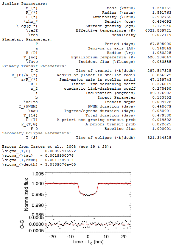
Ultimately, though all outputs are given, the only ones that are relevant right now are the transit time and duration. As these are observables, rather than calculated parameters, these values do not strongly depend on the priors or the modelled system parameters.
Here is the list of transit times and durations for all transits. Transits 15 and 20 were not modelled, as stated before, but they are given spaces in the list for completeness. All values are given in units of days.
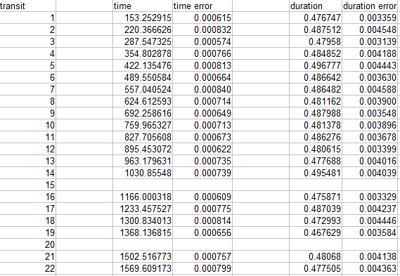
And here is the same table, in plain text:
transit time time error duration duration error
1 153.252915 0.000615 0.476747 0.003359
2 220.366626 0.000832 0.487512 0.004548
3 287.547325 0.000574 0.47958 0.003139
4 354.802878 0.000766 0.484852 0.004188
5 422.135476 0.000813 0.496777 0.004443
6 489.550584 0.000664 0.486642 0.003630
7 557.040524 0.000840 0.486482 0.004588
8 624.612593 0.000714 0.481162 0.003900
9 692.258616 0.000649 0.487988 0.003548
10 759.965327 0.000713 0.481378 0.003896
11 827.705608 0.000673 0.486276 0.003678
12 895.453072 0.000622 0.480615 0.003399
13 963.179631 0.000735 0.477688 0.004016
14 1030.85548 0.000739 0.495481 0.004039
15
16 1166.000318 0.000609 0.475871 0.003329
17 1233.457527 0.000775 0.487039 0.004237
18 1300.834013 0.000814 0.472993 0.004446
19 1368.136815 0.000656 0.467629 0.003584
20
21 1502.516773 0.000757 0.48068 0.004138
22 1569.609173 0.000799 0.477505 0.004363
This is getting long, so I'm gonna split this into multiple comments…
Posted
-
by
Shellface
in response to Shellface's comment.
Continuing:
To get to study the TTVs, the times must be compared to an orbital period in order to determine their difference from a linear ephemeris. First, I used the catalogue period of 67.595 days. The observed - calculated values for the transit times were plotted against their transit numbers, like so:
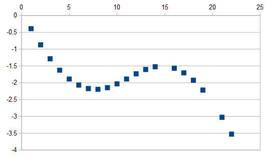
The y-axis is in days. It can be seen that this period is close to correct, but could use improvement; the observed transit times become earlier than expected increasingly over time, though the times are clearly modulated by a large sinusoid as well. Since we are plotting transit time minus the number of periods elapsed against time, the first derivative of this is a change in transit time over time, which in more sensical terms is a change in period (the second derivative would be a change in period over time, which is what TTVs are, in a round-about way). Since the derivative is negative, the period will need to be decreased. Fitting a linear trend + sinusoid solution gives a best-fit period of 67.4151 ± 0.0082 days, which should be mostly correct in absolute terms.
Using this new period, an improved plot of observed - calculated times against transit number can be made. It is shown below:
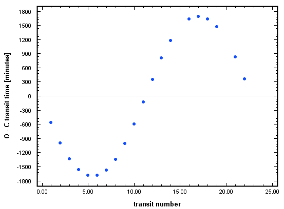
Note that the y-axis is now in minutes. It is now clearly visible how large the TTVs are; 1 day is 1440 minutes, so the semi-amplitude of the TTVs is about 1.2 days. These are, by far, the largest sinusoidal TTVs observed on any Kepler target that I know about - for comparison, as a proportion of the orbital period, TTVs of this amplitude would make an Earth year change by almost two weeks. The error bars are actually plotted on the above diagram, but as they are all around 1 minute, they are far too small to be discernable.
As the TTVs appear to be dominated by a single signal, a 1-sinusoid fit is attempted to start off with. The fit is reasonably good, but significant residuals can be seen:
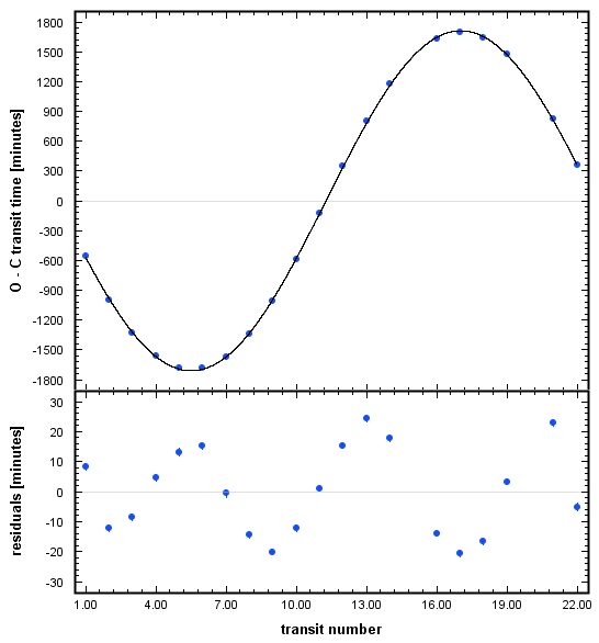
Though this could, in principle, be due to a third planet interacting with the transiting one, I am more inclined to believe that this is either due to the "chopping" signal with the companion causing the major super-period in the transit times, or possibly due to the period of the other companion being close to another resonance (the period is shorter and the amplitude smaller, which are both consistent with a more distant resonance). As the excess variations appear to be sinusoidal, too, a 2-sinusoid fit is used to model them out. This fit is better; though there are still residuals, they do not appear to be particularly orderly. They may represent stochastic variations due to quasi-random gravitational interaction.
The fitted sine waves have periods of 22.97 ± 0.59 and 7.52 ± 0.53 orbital periods, and semi-amplitudes of 1.209 ± 0.057 and 0.0142 ± 0.0023 days, respectively. The absolute periods are thus 1549 ± 40 and 507 ± 36 days. The shorter period is 1/3rd of the super-period to well within one sigma; this is mildly supportive of the two signals being due to one companion being close to two resonances, and though it should be possible to use this information to solve which resonances they are, it is excessively difficult without any prior information. As the smaller signal has approximately 1/85th of the amplitude of the larger one, it is probable that the larger signal is due to a low-order resonance, so the smaller one would have to be a high-order one (or alternatively, a very distant low-order one), of which there are very many. Ultimately, it is not worth attempting to solve this manually; a computer would be far better suited for the job. And, of course, this extra variation could be due to chopping, which I do not know any equations for, and is thus much better suited for a computer, too.
On a similar note, though, it is feasible to give mass estimates for the second companion if we assume which resonance it is in to cause the large-amplitude variations. Due to the large amplitude it is probably low-order, but the lack of observed transits suggests that the period ratio is probably not too low. Following the equations of Lithwick et al. (2012), here are tables of solutions for some first order resonances:
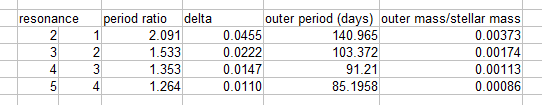
Where 2| 1 means 2:1. For the KIC stellar mass of 1.34 Msol, the implied masses are 5.2, 2.4, 1.6 and 1.2 Mjup, respectively, assuming zero eccentricity. These are quite reasonable; there are several long period, resonant giant planet systems that have been detected by RV surveys. Though it must be said that the system does not have to be in any of these resonances, it at least gives some confidence that this can be a resonant planetary system.
This is about as far as I can really study the transit timings, given my lack of ability to analytically analyse this stuff. We can briefly turn to the transit durations, though they do not follow any particular equations like TTVs do, so only broad, qualititive inferences can be made without analytical study. The transit durations are plotted below:
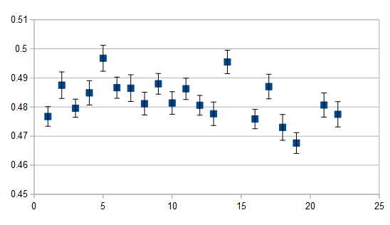
Where the y-axis is total transit duration in units of days. There appears to be a slow drift in durations, with a gradual increase up to transit ~6, then a similar decrease through the rest of the data, as well as sporadic jumps in duration at various times. Again, ultimately, not much can be inferred from this to the eye, but I am confident these will be valuable for solving the interactions of this system analytically.
What I can do, however, is analyse the transits; as we now know each transit's deviation from a linear ephemeris, if each transit lightcurve is shifted to correct for this the resulting lightcurve can be treated as a version of the lightcurve "corrected" for TTVs, though this ignores the (relatively small) error on the transit times and assumes constant durations (which is a decent approximation, as the TDVs are not too large). I fed this de-TTV'd lightcurve into EXOFAST with the same priors as before except for the improved value of the orbital period (67.4151 d); note that the output will have this period by design because the data has been forced to this period. The output is shown below:
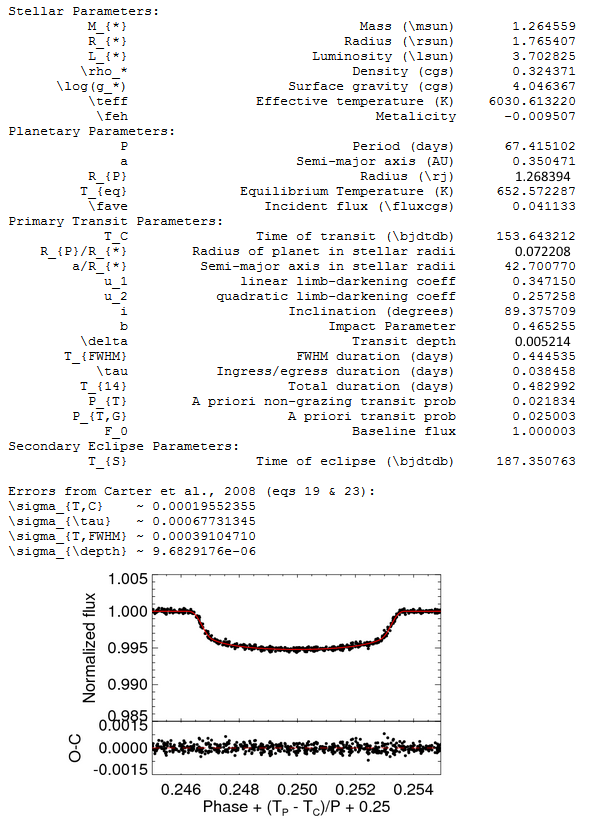
As usual, EXOFAST underestimates the transit depth; values relating to it have been corrected manually.
The model seems to have a fairly strong bound on the impact parameter - using priors in an attempt to force it take values of ~0 still results in output values of ~0.4. Thus, the errors on the inclination and the stellar density should be small.
It is remarkable that the calculated stellar radius is essentially exactly the same as the lower limit derived previously (>~1.76 Rsol); this is strongly supportive of spin-orbit alignment. Observations of the planet's Rossiter-Mclaughlin effect could be used to confirm this result.
Finally, it is interesting to note that, despite having a relatively low equilibrium temperature - low enough that it should be cloudless, following Sudarsky's classifications - it has a radius of ~1.27 Rjup, which is larger than expected for a giant planet that is not particularly young. Planetary radius stops strongly responding to mass for masses above ~1 Mjup; the expected radius for a planet in this general range is 1.0 - 1.1 Rjup. Though Hot Jupiters often have radii larger than this, that is due to their large incident fluxes; it seems another explanation is necessary. As the star is beginning to evolve, it must be several Gyr old, so the planet must be as old as well, so youth is not a valid explanation. It seems unlikely that resonant interactions can impart so much energy into the planet. I cannot give a strong explanation, but it may be explainable with some further study.
This looks like an extremely interesting system for study of dynamical interactions of giant planets, something rarely seen via transit. I am optimistic that the photometry can be used to solve the planetary parameters with appropriate modelling. Let's see that done!
Posted
-
 by
ajamyajax
in response to Shellface's comment.
by
ajamyajax
in response to Shellface's comment.
KIC 9032900 KOI 134: using your TTV values, I saw no sign of an EB in an alternating fit (even tried a half period TTV plot). It sure looks like a planet though.
But apparently some time ago the team who authored this paper decided this looked like a spectroscopic binary. ?? Also some related comments and links that might interest a bit.
table entry:
134.01 9032900 86.18499 67.179946 5056 167 SB1
SB1 Single-line eclipsing binary star. RV varies by over 1 km/s in low SNR reconnaissance spectra. Double lines not seen.
from:
"Characteristics of planetary candidates observed by Kepler, II: Analysis of the first four months of data"http://arxiv.org/ftp/arxiv/papers/1102/1102.0541.pdf
from:
http://en.wikipedia.org/wiki/Spectroscopic_binary#Spectroscopic_binaries"In (spectroscopic) systems, the separation between the stars is usually very small, and the orbital velocity very high. Unless the plane of the orbit happens to be perpendicular to the line of sight, the orbital velocities will have components in the line of sight and the observed radial velocity of the system will vary periodically. Since radial velocity can be measured with a spectrometer by observing the Doppler shift of the stars' spectral lines, the binaries detected in this manner are known as spectroscopic binaries. Most of these cannot be resolved as a visual binary, even with telescopes of the highest existing resolving power."
"In some spectroscopic binaries, spectral lines from both stars are visible and the lines are alternately double and single. Such a system is known as a double-lined spectroscopic binary (often denoted "SB2"). In other systems, the spectrum of only one of the stars is seen and the lines in the spectrum shift periodically towards the blue, then towards red and back again. Such stars are known as single-lined spectroscopic binaries ("SB1")."
marcy on CFOP
2012-01-05 22:44:26"The eclipse period of P = 67.18 d, and the huge transit time variations (17 hours), suggest a triple system, with one of the companions having P = 67.2 d and the other coming close enough to the primary to tidally spin it up. "
"Alternatively the transits are caused by a planet (not a star) having P = 67.2 d in an eccentric orbit that performs the tidal spin-up at periastron. If so, there would need to be a third orbiting object causing the transit-time variations."
" Is this really a false positive? The transit depth of 0.995 suggests planet size of ~0.9 R_JUP, not necessarily stellar. (But it could be an M dwarf.) I wonder if the transit period of P=67.18 d is actually caused by a planet and its "TTV" of 17 hours is caused by a third object. One of those two orbiting objects would still be needed to tidally spin-up the primary star to Vsini = 18 km/s."
"Red Giants in Eclipsing Binary and Multiple-Star Systems: Modeling and Asteroseismic Analysis of 70 Candidates from Kepler Data"
Patrick Gaulme, Jean Mc Keever, Meredith L. Rawls, Jason Jackiewicz, Benoit Mosser, Joyce Guzik
http://arxiv.org/abs/1303.1197
Posted
-
by
Shellface
in response to ajamyajax's comment.
Yes, I have seen all that. I have a few years of experience with spectroscopy and radial velocities - more than photometry, really - and this does not look like a spectroscopic binary. I imagine the SB1 designation refers to the two Lick recon spectra (see the earliest CFOP comments), which showed large RV variations, but it was later determined that one of the spectra was from another star, which invalidates the result. Notably, the TRES spectra indicate no RV variability over a few hundred m/s, an amplitude in the upper planetary range. I will stand by my previous statement that the only plausible solution is a planetary companion.
Also - I disagree with Marcy's comment about how the star's v sin i seems overly high - this is not a strongly evolved star, and it has not increased in radius much from the main sequence - so its angular momentum (which directly translates to v sin i) is not much lower than when it was on the main sequence. However, its surface magnetism could have decreased significantly due to the changes in atmospheric structure, which can explain the lack of Ca II emission. Thus, the high rotation and low chromospheric activity are not exactly in conflict, and I would not use them as a basis for imparting such extravagant, unlikely and likely unstable solutions to the system.
I will also say that, though the star is a moderately fast rotator, it is not entirely unamenable for RV observations; a precision of <100 m/s is not infeasible. Though this is not all that favourable for the planetary RV amplitude (for 1 Mjup, K = 43 m/s, and RV amplitude scales linearly with companion mass for mass ratios close to zero), it is optimistically within useful ranges for observation of the planet's Rossiter-McLaughlin effect, which I have touched on previously.
Have you had any luck with TTVFast? I am optimistic that this is a system where the TTVs can unambiguously (or, at least with limited ambiguity) solve the extra companion parameters.
Posted
-
by
ajamyajax
in response to Shellface's comment.
Yes Yes, my TTVFast work continues... And I am optimistic as well, but if I have to figure it all out by myself (which is fine), could also take me a while. Of course I will post more results if (or when) I get to that stage because this is such a fascinating new area of study. 😃
Also FWIW, the bubble here is R_sol = 1.765407 and R_jup = 1.268394 plotted on my confirmed planets probability matrix. Even so, this could still be a planet. For reference the other studied systems in this region are:
pl_hostname,pl_massj,pl_radj,st_mass,st_rad
KELT-2 A 1.52200 1.286 1.31 1.83
HAT-P-7 1.77600 1.342 1.47 1.84
Kepler-87 1.02000 1.204 1.10 1.82
HAT-P-49 1.73000 1.413 1.54 1.83
CoRoT-26 0.52000 1.260 1.09 1.79
p.s. and just having a little fun with 'KOI 134 b' since my plot file doesn't like the text 'KOI 134.01'... Seriously though, I hope you have helped the PC chances here again with your work.
Posted
-
by
ajamyajax
Also what are the chances this could be a circumbinary system? Maybe that could explain the TTV dynamics and the SB1 observations.
(correction: scratch this, if your previous comment is correct about the SB being invalidated; sorry one of those memory days)
Posted
-
by
Shellface
in response to ajamyajax's comment.
Good to hear. I would be eager to help where necessary.
I think more appropriate axes for a plot here would be planetary radius against (planetary) equilibrium temperature. Planetary radii for giant planets are increased by high irradiation, which is directly relatable to their temperature. I expect the relationship between planetary radius and stellar radius for giant planets in the above plot is because most of those planets are Hot Jupiters which mostly lie at similar semi-major axes, so their irradiation becomes related to stellar luminosity, which is related to stellar radius. Plotting planetary radius against equilibrium temperature effectively cuts out the middle man.
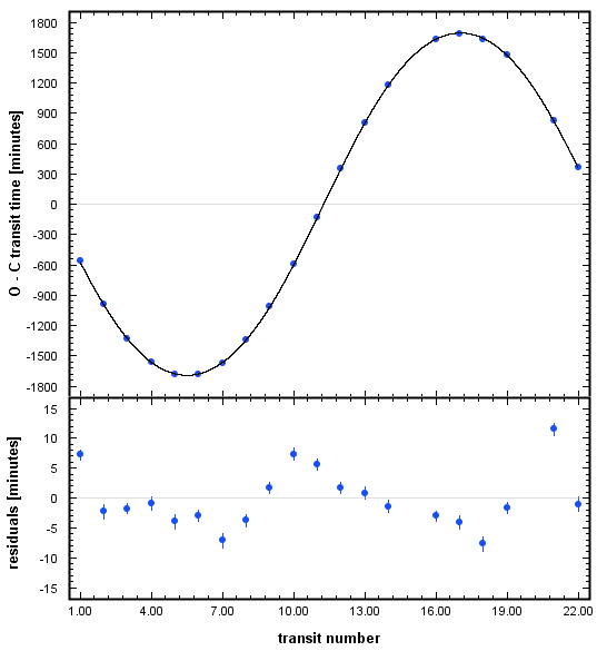
Today I realised that including a linear trend to the 2-sinusoid TTV model, which I did not consider the first time, yields a decent improvement to the fit. Here it is:

Though this may be over-fitting, I have no way to account for this and a proper model would be able to account for it anyway.
This new model implies an orbital period 17.5 ± 8.5 minutes shorter the previously given value, so the new new orbital period is 67.4029 ± 0.0059 days. As this is a change of 0.018%, this has little effect on previous calculations. The sinusoids now have periods of 23.62 ± 0.32 and 7.89 ± 0.36 orbital periods = 1592 ± 22 and 532 ± 24 days, and have semi-amplitudes of 1.273 ± 0.040 and 0.0164 ± 0.0020 days, respectively. The change in the amplitude of the super-period means a change in second companion mass of ~5%, which is little more than the 1 sigma errors. The observed period ratio of the sinusoids is 2.992 ± 0.090, consistent with 3:1 ratio.
I briefly checked whether the minor sinusoid was consistent with a distant a distant first-order resonance, but none of the values for the period ratio looked consistent with any value for the super-period - even when considering periods less than perfect resonance - so it seems that the minor period is probably not due to a first-order resonance. Again, computational modelling will be needed to solve the complexities here.
Posted
-
by
ajamyajax
in response to Shellface's comment.
Well I am still stymied today by the TTVFast inputs I posted before, so if you get any specific ideas there would appreciate the help.
But the other chart you mentioned was fairly easy to generate. Here are a few notes: only 214 of the 1854 entries currently in the confirmed planets table have pl_radj and pl_eqt column data. And the KOI 134 'b' display uses your 652.572287 K value (/1000). Also I limit the ranges to ymin = 0.05 ymax = 1.85 and xmin = 0.2 xmax = 2.55 just to make the plot clean and more readable (and resized the image larger as well). It is still most of the data. Hope this helps.
(chart update: axes reversed)

Data Credit: NASA Exoplanet Archive which is operated by the California Institute of Technology
Posted
-
by
ajamyajax
in response to ajamyajax's comment.
Update: good news, just checked my e-mail and heard back from Kat Deck who is travelling and speaking but promised to help us after that with TTVFast. So fingers crossed and all that. 😃
Posted
-
by
Shellface
I did leave a comment in the other thread, dunno if you saw it. Admittedly it's probably not enough, but it ought to be a step in the right direction!
Thanks for the improved plot. Though the axes should be reversed (radius is a function of eqiulbrium temperature), that is quite pedantic as the plot is perfectly understandable. It does look like KOI-134 b is somewhat inflated, though there is certainly a lack of low-insolation values for giant planets. I would like to study some of the long-period giant PC KOIs for a few reasons, and I suppose I should add "finding the normal radius for cool giants" to that list… hmph.
I suppose it does suggest that the stellar radius may be over-estimated, which generally implies an overestimated impact parameter, but as I said the fitted impact parameter seems quite secure. Unless we invoke something exotic like planetary rings at a peculiarly small seperation, it really does seem like the planet is inflated. I'm really stumped on how that could be possible… hmph.
Posted
-
by
ajamyajax
in response to Shellface's comment.
Yeah, saw that but need more specifics. But will keep working on it anyway.. Also, reversed the axes on that chart which hopefully improves the readability.
And should also mention: neat and effective O-C plots by you as well.
Posted
-
by
Shellface
More revisions: after looking at TTV systems with detected chopping signals, I notice that the signal period tends to be similar to the orbital period. I suspect that I have thus been modelling an alias of the chopping signal, following
Pl^-1 - 1 ≈ -(Ps)^-1, where "Pl" and "Ps" denote "long" and "short" periods.
…probably. Using the value for Pl given previously (7.89 orbital periods) gives Ps ≈ 1.145 orbital periods, which compares to the observed value of 1.140 ± 0.007 periods. Because these are aliases we are discussing, the goodness of fit and the amplitude of variability are pretty much unchanged, so previous value of 0.0164 ± 0.0020 days for the semi-amplitude remains correct.
If the interpretation of the extra signal as chopping is correct, then it can solve the system parameters when used in conjunction with the observed super-period. Unfortunately, the equations for chopping are wayyyy above my maths-think capabilities (see, for example, Deck & Agol (2014)), so I'm not up for it. However, since chopping was important for solving the parameters of PH3, I'm gonna posit that someone who might read this at some point can do something with this. Hopefully.
Posted
-
by
ajamyajax
Well FWIW -- and possibly in support of an unseen outer planet here, I tried running some of your outer periods through TTVFast and got results that were somewhat correlated. And still rough of course, but adding eccentricity values seem to make them 'almost' work. What do you think?
Outer period (days), Outer mass/stellar mass, (period object with eccentricity change)
140.965, 0.00373, P=67.415102, e=0.042
103.372, 0.00174, P=67.415102, e=0
91.21, 0.00113, P=91.21, e=0.02
85.1958, 0.00086, P=85.1958, e=0.035 (corrected)


TTVFast credit: Deck, Agol, Holman & Nesvorny, 2014, ApJ, 787, 132, arXiv:1403.1895
Posted
-
by
Shellface
in response to ajamyajax's comment.
Seems like things are in the right ballpark. Good work.
I did send Deck an email some days ago, but haven't received response yet.
Also, I've been quiet here because I've been fighting to understand some phase curve stuff in some K2 EB. That's mostly sorted, so I should be doing some planet stuff soon.
Posted
-
by
ajamyajax
in response to Shellface's comment.
SF, just wondered if you tried EXOFAST on the NEA yet?
https://exoplanetarchive.ipac.caltech.edu/docs/exonews_archive.html#20July2017
Posted
-
by
Shellface
in response to ajamyajax's comment.
I have tried it out. It doesn't seem appreciably different to I was using before, at least currently, but I will keep an eye on it.
Posted
-
by
ajamyajax
in response to Shellface's comment.
Nice, glad it works in a similar fashion anyway. I'll have to read thru your previous EXOFAST posts and figure out how to do that also sometime (probably be a while though).
Posted